Computer Aided Simulation of Dispersion Theory Based on Experimental
Data by Zone Circulating Flow-Injection Analysis
Yoshio NARUSAWA* and Yuichi MIYAMAE
 Return
There are so many investigations before 1980 on dispersion in laminar flow.1)~16) Yu17) studied the dispersion of a small quantity of a solute initially injected into a round tube in which steady-state laminar flow exists. Vrentas and Vrentas18) developed an asymptotic solution for the dispersion of a passive solute in a Newtonian fluid in fully developed, laminar flow through a straight, circular tube. Daskopoulos and Lenhoff19) studied the axial dispersion coefficient in laminar flow in a tube and pointed out that the dispersion is generally smaller in a curved tube than in a straight tube, because of the enhancement of lateral transport by secondary flows.
Mansour20) solved an exact, closed-form solution of a mathematical model describing the trans-port of solution matter in a solvent inside a circular tube in terms of a confluent hypergeometric function and showed to be in excellent agreement with published experimental and numerical works. Shankar and Lenhoff21) pointed out that the axial dispersion of an impulse tracer injected into a fluid in a flow in a tube is caused by the interaction of radial diffusion and the nonuniform velocity profile.
In relation to flow injection analysis, many investigators reported on the dispersion in laminar flow. Vanderslice et al.22) derived expressions for the dispersion and the travel times of samples in single flow-injection analysis systems. Ramsing et al.23) proposed the study on the highly reproducible concentration gradients formed between an injected sample zone and the carrier stream in flow injection analysis for titration based on measuring the time span between points of identical gradient dispersion. Riley et al.24) reported an alternative approach to analysis. Reijn et al.25) studied the dispersion of an injected sample zone caused by transport phenomena in most flow injection analysis systems. Betteridge et al.26) studied dispersion and chemical reaction in a single-channel flow-injection system modeled by a random walk method.
Vithanage and Dasgupta27) studied controlled dispersion with multidimensional spectral detection. Kristensen et al.28) studied on voltammetric microelectrodes with a total tip diameter of approximate 20um to probe dispersion in a simple flow-injection analysis system. Melnik and Fejes29) reported a review with 25 references concerning theoretical solutions of dispersion in flow-injection analysis and methods for suppression of axial dispersion. Stults et al.30) reported experimental studies on the effect of temperature on dispersion in a flow-injection system.
Zagatto et al.31) reported that the addition of a confluent stream increased the mean length of the sample zone and simultaneously decreased the involved concentrations. Kolev and Pungor32) investigated single-line flow-injection systems with two types of reactor with different disper-sion characteristics. Toei33) developed a multifunction pump delivery system with which any flow patterns were easily programmed and investigated the potential of the flow-gradient function in flow-injection analysis. McGowan and Pacey34) studied the effects of increasing internal diameters of coiled tubing in large-bore systems. Stone and Tyson35) studied the application of 2 models based on the stirred mixing tanks, the well stirred tank and the 2 tanks in parallel models. Muller and Kramer36) investigated the factors affecting the dispersion obtained in a flow injection system. Brooks and Rullo37) studied on the minimal dispersion flow injection analysis systems for automated sample introduction. Ilcheva and Dakashev38) developed the research on two-electrode cell for constant-potential coulometric detection in flow-injection systems.
Chung and Ingle39) proposed a new procedure for obtaining analytical kinetic information in a single-line flow-injection analysis system. Johnson et al.40) studied the reduction of injection variance in flow-injection analysis. Van Staden41),42) investigated the response time phenomena of coated open-tubular solid state silver halide selective electrodes and their influence on sample dispersion in flow-injection analysis. Korenagav43) studied solute dispersion of an injected sample plug by using an experimental apparatus with ideal laminar flow in order to develop a hydrodynamic model for the design of sensitive and precise flow-injection analysis systems.
Wentzell et al.44) investigated the evaluation of dispersion profiles by using random walk simulation in flow injection analysis. Studies are limited to the case of dispersion in straight tubes with laminar flow and no reaction.
Rios et al.45) applied multidetection in unsegmented flow systems with a single detector to chemical reaction. Kuroda et al.46) applied also the multidetection to simultaneous determination of iron(II) and (III). Li and Narusawa47),48) studied experimentally the sample zone dispersion in laminar flow by using zone circulating flow injection analysis (ZCFIA). There are three main by B bibliographies by Ruzicka and Hansen49), by Varcarcel and Luque de Castro50), and urguera (editor)51) on dispersion in relation to flow injection analysis. The present aim is to clarify quantitatively the relationships among dispersion coefficient and many FIA parameters by simulating the equations obtained earlier.47),48)
Dispersion Model
Ideal flow model and equations of injected sample zone in a tubular reactor
First, the ideal flow model of the injected sample zone in FIA system without containing a chemical reaction is shown in Fig. 1. By analyzing the model, the following equations (1)-(10) are derived. In these equations, L is a length (cm) of the tubular reactor; Lr is a traveled distance (cm) of the injected sample plug making physical dispersion and Ls is a plug width (mm) of the sample injected at a split second. Consequently, Ls obeys the following equation:

where Sv ( l) is the injected sample volume, r (mm) is the radius of the reactor. Lm, f (cm) is the dispersing distance of the injected sample plug forward and backward in the axial direction caused by molecular Brownian motion, and then it can be expressed by the equation:

where, Qm (cm3/s) is volume of molecular dispersion per second, and associates with viscosity of the carrier and diffusion coefficient of the sample molecule. t (s) is elapsed time, that is, the time of the sample zone dispersing after injection, and T is the residence time of the sample zone.
Therefore, the following equations can be established:


where the  is a peak width expressed with time elapsed of the sample zone from injection to the detector.
  is a dispersing width expressed with time elapsed of the injected sample zone because of molecular Brownian motion.
  is a width of the sample plug expressed with time;52) if the unit of the r is in millimeter on the chart, the peak width will be represented by the symbol of a (mm). The relationship between the
  (s) and (mm) can be expressed by the equation (mm) = a (s), in which, " a " is calculated from the recorder chart speed and is a constant. In this experiment, " a " was set to 6mm/s. When the traveled speed of the sample zone equals to that of the recorder chart, will equal to Ls , on ordinary occasions, the following equation is established:

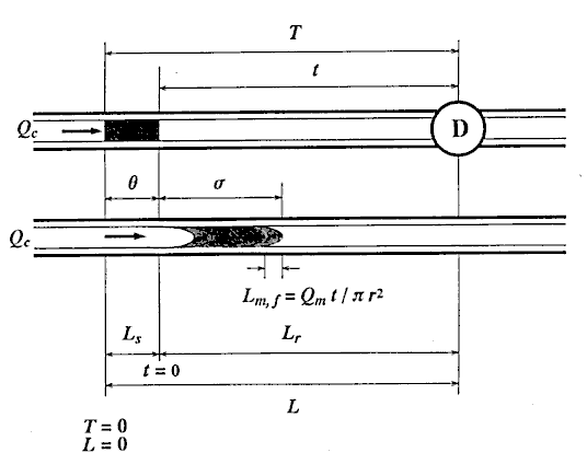
here, Qc (cm3/s) is the volumetric flow rate of the carrier stream, relates to the process of the convection of the injected sample plug and the Q is the total flux of the sample zone during traveling. Consequently:

From these definitions, following equations can also be derived:


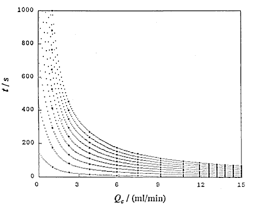
Second, the correctness of these equations was confirmed by the following experimental data obtained. That is the relationships of t against Lr were obtained from damped response curves under ten steps of the flow rate Qc , 1.02, 2.25, 3.80, 5.84, 7.39, 9.03, 10.7, 11.9, 12.6 and 13.2 ml/min. By analyzing linear regression, an equation of t = b Lr was obtained at each constant Qc.
Consequently, by using this equation, the relationships between Qc and Lr under 24 steps of time t from 20 to 250 s with every 10 s were obtained.
Experimental
Preparations of sample and carrier solution
Preparation of a carrier solution: Ultrapure water was used for the preparation of the solution. In this experiment, bubbles dissolved in a carrier solution became easily evolved as the revolution speed of a pump was accelerated. Therefore, degassing was made by the following manner, because the bubbles disturbed the determination of the sample injected. By using a membrane filter (pore size 0.45m), the carrier solution was filtrated under reduced pressure, and then the vessel containing the carrier solution was put into a supersonic cleaner to deeply degas.
The operation was continued until bubbles in the solution hardly evolved.
Preparation of a sample solution: Potassium dichromate was heated 2 hours at 110C in an electric oven. A potassium dichromate solution was prepared by dissolving 0.4000g of it into a 500ml volumetric flask and diluting to 500ml with water. The sample solution thus prepared was orange in color and 800ppm potassium dichromate having maximum wave length at 440nm.
Apparatus: Soma S-3250 single-beam spectrophotometer equipped with flow cell (inner volume 8l, path length 10mm) was used. Denki Kagaku Keiki (DKK) mini-pulse 5 channel peristaltic pump of multi-step revolutions, DKK single-channel injection valve and System Instruments Co. (SIC) chromatocorder-12 were also used.
Relationships between pump's revolution speeds and carrier stream's fluxes
A measurement method of pump revolution speeds (R) versus the volumetric flow rates of the carrier stream (Q) and the calibration method of the flow rates to the scales of the pump's revolution speed were referred to the literature cited.47),48) The pump revolution speed was in proportion to the volumetric flow rate of the carrier stream.
Procedure for detecting damped curves with ZCFIA method
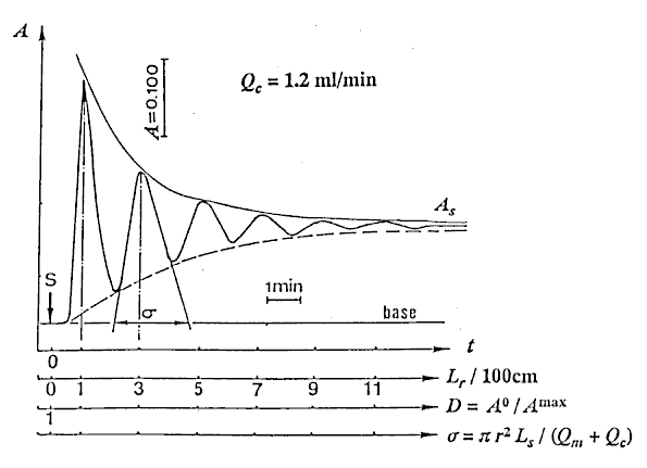
At first, the reproducibility test of the instrument was performed with the sample (Sv = 100l) by repeating measurement eleven times. The RSD was less than 0.5%. Next, water as carrier stream was pumped into the tubular reactor, simultaneously, the sample solution was aspirated into a loop by the pump, and then the pump was stopped. After connecting the inlet of the carrier to the outlet of the waste in the single line manifold keeping away from bubble entering, the valve was switched from the load position to injection position. Then, the pump and the recorder were started at the same time, and the determination of the injected sample was started. 12 minutes needed for determining one time. The results detected were a set of damped response curves. The initial peak is attributed to the result of the injected sample zone traveled only 100cm. As the closed-flow system has the total length (L) of 200cm, the peak of the damped curve will appear at every 200cm distances until it completely homogenized. The number of the peaks obtained coincides with the number of times that the zone passes through the detector. The sample zone diffuses as traveling forward, and the peak heights fall down with increasing in residence time (T). Lastly, the detector signal (absorbance A or height H) changes to a plateau of steady state due to the complete mixing of the sample zone by the carrier. In order to correlate H with the dispersion coefficient (D), H0 is detected by letting the sample solution flow through the detector instead of the carrier stream. The H0 was obtained to be 23.6cm in this experiment.
Typical damped response curve obtained at Qc = 1.2 ml/min is shown in Fig. 2.
Results and discussion
Correlations between Q, L, T, r, Sv and D
The dispersion coefficient D has been defined as the ratio of concentrations of sample material before and after the dispersion process has taken place in that element of fluid that yields the analytical readout. Because the height indicated with H (cm) of the peak of output signal is proportional to the concentration of injected sample Cmax, D may be expressed as the following equation:

The numerical values of D were obtained by substituting Hmaxs of the peak heights being existed in Fig. 2 into the equation (11).
Connecting each peak of the damped curve with the smoothed curve as shown in Fig. 2, H values at each instant time from 20 to 250 with every 10 seconds were obtained under 10 steps of flow rates mentioned above. And substituting H for Hmax into Eq. (11), values of dispersion coefficient D at each instant time were also obtained.
Computer aided simulation
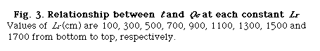
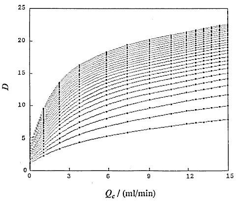
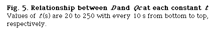
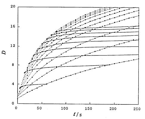
Using UBASIC program,53) the following three relationships were obtained: that is t and Lr at constant Qc (DIM 2), t and Qc at constant Lr (DIM 10, Fig. 3), and Lr and Qc at constant t (DIM 2, Fig. 4).
Next, the following five relationships between dispersion coefficient D and FIA parameters:
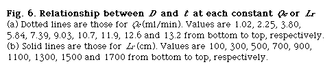
that is, D and Lr at constant Qc (DIM 7), D and Qc at constant Lr (DIM 7, Fig. 5), D and Qc at constant t (DIM 7), D and t at constant Qc (DIM 7, Fig. 6 (a)) and D and t at constant Lr (DIM 7, Fig. 6 (b)). Symbol DIM means dimension of the matrix in the curve-fitting program, and DIM-1 corresponds to the order of polynomials. Therefore, DIM = 2 means the relationship is the linear regression.
Molecular dispersion
A group of the plots of Lr against Qc was obtained as shown in Fig. 4. It is observed that even if the Qc is nought, Lr is not nought and the intercept increases with increase in residence time (t). If analyzing the phenomenon, it may be thought that the intercept comprises the length of the injected sample plug (Ls) and the diffusion distance (Lm, f) caused by molecular dispersion of the sample plug. On the other hand, according to the equation (10), if Qc is decreased to nought, the following equation can be derived:

where Lm, f is positive and increases as the time t increases. Fig. 4 shows that the intercept at Qc = 0 represents the value of Lm, f . That is, the theory predicts the same conclusion as the experimental result.
Analytical expression of dispersion
Analyzing these curves concerning Qc , Lr and D, the following mathematical expression was obtained.
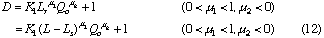
where, K1 is a constant, u1 and u2 are also constants but the values will change with differences in experimental conditions in some definite ranges.
Correlations between dispersion coefficient of the sample zone and the volumetric flow rate of the carrier stream were obtained. Consequently, the following expression similar to the expression (12) is again obtained:
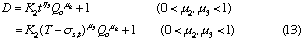
where, K2 is a constant, and u3 is also a constant under the limited conditions.
If the volumetric flow rate of the carrier stream, the length and inner diameter of the reaction coils, and the injected sample volume are not changed, the data about correlations between the residence time and dispersion coefficients of the injected sample zone will be found. As a result, those data were obtained under various conditions of Qc and t. By analyzing those data, the following expression was also obtained:
where, K3 is a constant.
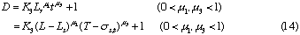
In addition, if the Eq. 1 is substituted into the expressions (12) and (14), the following expressions will be further deduced:
From the expressions (8), (9), (10) and (14), the following expressions are also obtained:
Computer aided simulation for dispersion theory
(a) Relation of dispersion coefficient D with the length of tubular conduit Lr and the volumetric flow rate Qc
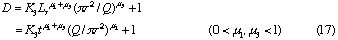
By taking logarithm of D subtracted by 1 in Eq. (12), we obtain the following equation.

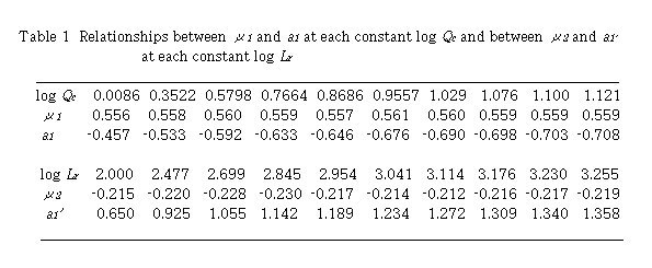
By plotting log (D - 1) against log Lr at each constant Qc , linear relationships were obtained. Slopes of these curves give  and intercept a1 gives log K1 +
  log Qc. Results are shown in Table 1. Mean value of is 0.559 + 0.002. By plotting a1 against log Qc , was obtained from the slope and log K1 was obtained from the intercept. Values of and log K1 were obtained to be -0.224 and -0.457, respectively. Regression coefficient r = -0.9989. The intercept a1 showed a linear relationship against log Qc with negative slope. This means that u2 is negative and perspective of Eq. (12) on is reasonable.
Next, plot of log (D - 1) against log Qc at each constant Lr , linear relationships were obtained. Slopes of these curves give u2 and intercept a1' gives log K1 + log Lr. Results are also shown in Table 1. Mean values of is -0.219 + 0.006. Plotting of a1' against log Lr gave from the slope and log K1 from the intercept. Values of and log K1 were obtained to be 0.557 and -0.457, respectively. Regression coefficient r = 0.9996. The intercept a1' showed a linear relationship against log Lr with positive slope. Two sets of K1 , and coincided very well with each other.
(b) Relation of dispersion coefficient D with the volumetric flow rate Qc and the time t
By taking logarithm of D subtracted by 1 in Eq. (13), we obtain the following equation.

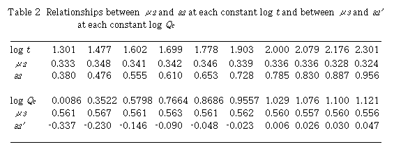
By plotting log (D - 1) against log Qc at each constant t, linear relationships were obtained. Slopes of these curves give and intercept a2 gives log K2 +  log t. Results are shown in Table 2. Mean value of is 0.335 + 0.009. By plotting a2 against log t, was obtained from the slope and log K2 was obtained from the intercept. Values of and log K2 were obtained to be 0.567 and -0.350, respectively. Regression coefficient r = 0.9996. The intercept a2 showed a linear relationship against log t with positive slope. This means that is positive and perspective of Eq. (13) on is reasonable. In addition, the intercept gives log K2.
Next, plot of log (D - 1) against log t at each constant Qc , linear relationships were obtained. Slopes of these curves give and the intercept a2' gives log K2 + log Qc. Results are also shown in Table 2. Mean value of is 0.561 + 0.003. Plotting of a2' against log Qc , and logK2 were obtained to be 0.343 and -0.346, respectively. The intercept a2' showed a linear relationship against log Qc with positive slope. The slope gives and the intercept gives log K2. Two sets of K2 , and coincided very well with each other.
(c) Relation of dispersion coefficient D with the length of tubular conduit Lr and the time t
By taking logarithm of D subtracted by 1 in Eq. (14), we obtain the following equation.

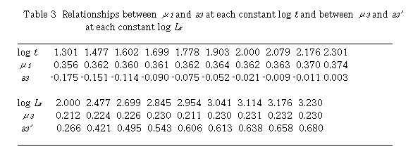
By plotting log (D - 1) against log Lr at each constant t, linear relationships were obtained. Slopes of these curves give and intercept a3 gives log K3 + log t. Results are shown in Table 3. Mean value of is 0.363 + 0.006. The intercept a3 showed a linear relationship against log t with positive slope. and log K3 were obtained to 0.186 and -0.409, respectively. Regression coefficient r = 0.9902. This means that is positive and perspective of Eq. (14) on u3 is reasonable. In addition, the intercept gives log K3.
Next, plot of log (D - 1) against log t at each constant Lr , linear relationships were obtained. Slopes of these curves give and intercept a3' gives log K3 + log Lr. Results are also shown in Table 3. Mean value of is 0.225 + 0.008. The intercept a3' showed a linear relationship against log Lr with positive slope. The slope gives u1 and the intercept gives log K3. Values of and log K3 were obtained to be 0.338 and -0.413, respectively. Regression coefficient r = 0.9983. Two sets of K3 , and coincided fairly well with each other.
Finally, the present paper realized quantitative conclusions for the analytical expressions from Eq. (12) to Eq. (16) by the computer aided simulation.
Conclusion
1: In FIA system, the interrelations among L, Q, T, r and Sv obey the equations (8), (9) and (10). When volumetric flow rate of the carrier stream is fixed, the residence time of sample zone would be proportional to the traveled distance of the sample zone; if the traveled distance of the sample zone is fixed, the residence time of it would be reciprocally proportional to the volumetric flow rate of the carrier stream; if the residence time is fixed, the traveled distance of sample zone would be proportional to the volumetric flow rate (or mean linear flow velocity) of the carrier stream; even if the flow of the sample zone stopped, dispersion of injected sample zone is continuously conducting and the dispersing distance of the sample zone is monotonously increasing with elapsing time of the carrier stopped.
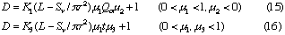
2: In FIA system, when volumetric flow rate of the carrier stream, inner diameter of the tubular reactor and injected sample volume are fixed, dispersion of the sample zone will increase with increase in the reactor length (cf. Eq. (12)). However, if the length and inner diameter of the tubular reactor, and injected sample volume are fixed, dispersion conversely decreases with increasing in volumetric flow rate of the carrier stream (cf. Eq. (15)).
3: In FIA system, if the residence time of sample zone, the inner diameter of the reactor and injected sample volume are fixed, the dispersion would increase with increasing in the volumetric flow rates of the carrier stream within narrow conduit system (cf. Eq (13)); if the volumetric flow rate of the carrier stream, the inner diameter of the reactor and injected sample volume are fixed, the dispersion would increase with increasing in the residence time of sample zone. Although this conclusion 3 may be in contradiction to the conclusion 2, this conclusion also holds under the restricted conditions. It is worthwhile to mention that to make qualitative correlations among the parameters of Q, L, T and D in FIA system without any definite conditions will mislead the conclusions.
4: According to above expression (cf. Eq. (14)) in FIA system, if the length and inner diameter of the reactor, and injected sample volume were fixed, the dispersion would also increase with increase in the residence time of the sample zone flowing through narrow conduit system; if the residence time of the sample zone and injected sample volume are fixed, the dispersion also increases with increasing in the length of the reactor.
5: In FIA system (cf. Eqs. (15) and (16)), if the length and inner diameter of the reactor, and the volumetric flow rates of the carrier stream (or the residence time of the sample zone) are fixed, the dispersion would decrease with increase in the injected sample volume. If the injected sample volume increases up to the total volume of the reactor, the value of the dispersion coefficient will approach to unity.
6: From the above expression in FIA system (cf. Eqs. (15) and (16)), if injected sample volume, the length and inner diameter of the reactor , and the volumetric flow rates of the carrier stream (or the travel distance of the sample zone) are fixed, the dispersion would increase with increase in the inner diameter of the reactor; besides, if the injected sample volume, the residence time of the sample zone and the volumetric flow rates of the carrier stream are fixed, the dispersion would reversely decrease with increasing in the inner diameter of the reactor.
The authors deeply thank Mr. S. Kitahama, Denki Kagaku Keiki Co., for his supply of the multi-step peristaltic pump used in the experiment and Mr. Y.-S. Li and K. Takahashi, Rikkyo University, for their assistance in some parts of the experiment. They also thank Nomura Microscience Co. for the supply of ultrapure water.
References
1) N. W. Gill, V. Ananthakrishnan, and R. J. Nunge, AIChE J., 14, 939 (1968).
2) C.-G. Wan and E. N. Ziegler, Chem. Eng. Sci., 25, 7236 (1970).
3) J. A. Guin, D. P. Kessler, and R. A. Greenkorn, Ind. Eng. Chem. Fundam., 11, 477 (1972).
4) M. Posner and W. N. Gill, AIChE J., 19, 151 (1973).
5) E. Gola, F. Avezzu, A. Marani, and A. Paratella, Quad. Ing. Chim. Ital., 8, 21 (1972).
6) E. Gola, A. Marani, F. Avezzu, R. Dabala, and A. Paratella, Quad. Ing. Chim. Ital., 9, 89 (1973).
7) R. N. Trivedi and K. Vasudeva, Chem. Eng. Sci., 30, 317 (1975).
8) L. A. M. Janssen, Chem. Eng. Sci., 31, 215 (1976).
9) G. S. Booras and W. B. Krants, Ind. Eng. Chem. Fundam., 15, 249 (1976).
10) K. D. P. Nigam and K. Vasudeva, Chem. Eng. Sci., 31, 835 (1976).
11) N. Rudraiah, Vignana Bharathi, 2, 1 (1976).
12) D. Pamda and V. V. R. Rao, Indian J. Technol., 14, 410 (1976).
13) G. R. Carbonell and B. J. McCoy, Chem. Eng. Commun., 2, 189 (1978).
14) M. R. Doshi, P. M. Daiya, and W. N. Gill, Chem. Eng. Sci., 33, 795 (1978).
15) J. H. M. van den Berg and R. S. Deelder, Chem. Eng. Sci., 34, 1345 (1979); 36, 1106 (1981).
16) P. K. Mayock, J. M. Tarbell, and J. L. Duda, Sep. Sci. Technol., 15, 1285 (1980).
17) J. S. Yu, J. Appl. Mech., 48, 217 (1981).
18) J. S. Vrentas and C. M. Vrentas, AIChE J., 34, 1423 (1988).
19) P. Daskopoulos and A. M. Lenhoff, AIChE J., 34, 2052 (1988).
20) A. R. Mansour, Sep. Sci. Technol., 24, 1437 (1989).
21) A. Shankar and A. M. Lenhoff, AIChE J., 35, 2048 (1989).
22) J. T. Vanderslice, K. K. Stewart, A. Rosenfeld, H. Gregory, and J. Darla, Talanta, 28, 11 (1981).
23) A. U. Ramsing, J. Ruzicka, and E. H. Hansen, Anal. Chim. Acta, 129, 1 (1981).
24) C. Riley, L. H. Aslett, B. F. Rocks, R. A. Sherwood, J. D. M. Watson, and J. Morgon, Clin. Chem. (Winston-Salem, N. C.), 29, 332 (1983).
25) J. M. Reijn, H. Poppe, and W. E. van der Linden, Anal. Chem., 56, 943 (1984).
26) D. Betteridge, C. Z. Marczewski, and A. P. Wade, Anal. Chim. Acta, 165, 227 (1984).
27) R. S. Vithanage and P. K. Dasgupta, Anal. Chem., 58, 326 (1986).
28) E. W. Kristensen, R. L. Wilson, and R. M. Wightman, Anal. Chem., 58, 986 (1986).
29) S. Melnik and J. Fejes, Chem. Listy, 81, 243 (1987).
30) C. L. M. Stults, A. P. Wade, and S. R. Crouch, Anal. Chim. Acta, 192, 301 (1987).
31) E. A. G. Zagatto, B. F. Reis, M. Martinelli, F. J. Krug, F. H. Bergamin, and M. F. Gine, Anal. Chim. Acta, 198, 153 (1987).
32) S. P. Kolev and E. Pungor, Anal. Chim. Acta, 208, 117 (1988).
33) J. Toei, Talanta, 35, 425 (1988).
34) K. A. McGowan and G. E. Pacey, Anal. Chim. Acta, 214, 391 (1988).
35) D. C. Stone and J. F. Tyson, Analyst (London), 112, 515 (1987); 114, 1453 (1989).
36) H. Muller and J. Kramer, Fresenius' Z. Anal. Chem., 335, 205 (1989).
37) S. H. Brooks and R. Rullo, Anal. Chem., 62, 2059 (1990).
38) . L. Ilcheva and A. Dakashev, Analyst (London), 115, 1247 (1990).
39) . H. K. Chung and J. D. Ingle, Jr., Anal. Chem., 62, 2547 (1990).
40) B. F. Johnson, R. E. Malick, and J. G. Dorsey, Talanta, 39, 35 (1992).
41) J. F. van Staden, Analyst (London), 117, 51 (1992).
42) J. F. van Staden, Anal. Chim. Acta, 261, 381 (1992).
43) T. Korenaga, Anal. Chim. Acta, 261, 539 (1992).
44) P. D. Wentzell, M. R. Bowdridge, E. L. Taylor, and C. MacDonald, Anal. Chim. Acta, 278, 293 (1993).
45) A. Rios, M. D. Luque de Castro, and M. Valcarcel, Anal. Chem., 57, 1803 (1985).
46) R. Kuroda, T. Nara, and K. Oguma, Analyst (London), 113, 1557 (1988).
47) Y.-S. Li and Y. Narusawa, J. Flow Injection Anal. (in Japanese), 10, 66 (1993).
48) Y.-S. Li and Y. Narusawa, Anal. Chim. Acta, in press.
49) J. Ruzicka and H. Hansen, " Flow Injection Analysis ", 2nd ed., John Wiley & Sons, New York, 1988.
50) M. Valcarcel and M. D. Luque de Castro, " Flow-Injection Analysis -- Principles and applications " , Ellis Horwood, Chichester, 1987.
51) J. L. Burguera (editor), " Flow Injection Atomic Spectroscopy ", Marcel Dekker, Inc., New York, 1989.
52) R. S. Schifreen, D. A. Hanna, L. D. Bowers, and P. W. Carr, Anal. Chem., 49, 1927 (1977).
53)Y. Narusawa and Y. Miyamae, J. Chem. Software (in Japanese), 1, 99 (1993).
Return