Discrimination of Marihuana Using Cluster Analysis

Syuji OKUYAMA and Toshiyuki MITSUI


Return

Introduction

Recently in Japan, marihuana, cocaine and opium are increasingly used as drugs instead of methamphetamine. In this paper, for presumption of the purchasing pathway to marihuana, the discrimination among marihuana was investigated using cluster analysis [1,2] and personal computer programing for the discrimination of some samples. We have already shown that cluster analysis is a powerful technique for the qualitative analysis of materials such as resins [3], medicines [4] and fibers [5]. The advantage of this method is that there is no bias from the interpreter. The calculation is completed using a personal computer without involving the prejudice of the analyst. Using this method, the characterization of each sample could be approximately estimated.
The discrimination was completed using 43 marihuana samples that were seized at the Aichi prefecture in Japan in November 1994. These samples were measured using gas chromatography (GC) and gas chromatograph mass-spectrometry (GC-MS). The obtained data were corrected as a fixed rule. Cluster analysis was performed using the corrected values. Discrimination among marihuana can now be investigated with taking into account the results of this cluster analysis.

Experimental

At first, 5 ml of n-hexane was added to 50 mg of marihuana and it was permitted to stand for ten minutes. The obtained solution was concentrated to 1 ml using a water bath at 90 oC, and 1 ml of concentrated solution was measured using GC and GC-MS. The GC peaks of cannabidiol (CBD), tetrahydrocannabinol (THC) and cannabinol (CBN) and some fragment ions of tetrahydrocannabivarin (THCV), CBD and THC using GC-MS were selected using quantification IV[2]. Using the selected peaks and fragment ions, the discrimination among the marihuana was performed using the cluster analysis. The quantification IV and cluster analysis were calculated using a personal computer (NEC PC-9801 RX) which was programed in Basic.

Investigation of the analytical conditions of GC and GC-MS

The optimum conditions for GC and GC-MS were selected according to reproducibility and operation times. The best analytical conditions of GC and GC-MS for the discrimination of marihuana are shown in Tables 1 and 2, respectively.

               Table 1  Operating conditions of GC/MS
              ------------------------------------------------
               Instrument           JEOL JMS-DX300
                                    MS-GCG05
               Column               1.5% Silicone OV-17
                                    (2.5mm i.d. x 1m)
               Column temp.         230C
               Injection temp.      250C
               Separator temp.      250C
               Inlet temp.          250C
               Chamber temp.        200C
               Ionization volt       70V
               Ionization current   300.micro.A
               Carrier gas          He 
              ------------------------------------------------ 
               Table 2    Operating conditions of GC
              -------------------------------------------------- 
               Insturument          HEWLETT PACKARD
                                    5890 SERIES II
               Column               DB1 (0.53mm i.d. x 15m)
               Column temp.         230C
               Injection temp.      250C
               Detecter temp.       250C
               Carrier gas          He 
              ------------------------------------------------- 

The effect of the reproducibility against the measurement result of the same sample for GC and GC-MS

The discrimination among marihuana is very difficult if each content of THCV, CBD, THC and CBN in marihuana varies with elapsed time and the degree of variation is random to elapsed time. Accordingly, each content of THCV, CBD, THC and CBN to different elapsed time in marihuana was investigated using the peak areas of GC and GC-MS. It was found that the measurement results were unchanged over three months.

Preparation of filed data

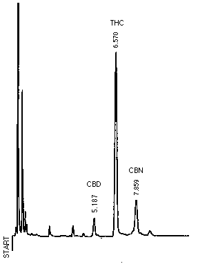
The peak areas of GC and GC-MS that were effective for cluster analysis from within all components in marihuana were selected using the quantification IV. The quantification IV is the method used for selecting data that would be useful in the cluster analysis and the specific peak areas of several components are selected for the discrimination of marihuana. This time, the three peaks for GC and eight mass fragment ions in the three components for GC-MS were selected and these peak areas were read out. The selected three peaks from the GC were CBD, THC and CBN, and the fragment ions from the GC-MS were 271, 243 and 231 in THCV, 231 in CBD and 314, 299, 271, and 231 in THC. The chromatograms of GC and GC-MS are shown in Figures 1 and 2. Even if the areas of the other GC peaks and fragment ions were larger than


Fig.1 Chromatogram of GC
CBD :Cannabidiol
THC :Tetrahydrocannabinol
CBN :Cannabinol


Fig.2 Total ion chromatogram of GC-MS
THCV:Tetrahydrocannabivarin
CBD :Cannabidiol
THC :Tetrahydrocannabinol

those of the selected peaks and fragment ions, they were hardly differentiated among marihuana and were not useful in the cluster analysis. In these selected peaks and fragment ions, THC for GC and 314 in THC for GC-MS were used as the internal standards. For GC, the areas of CBD and CBN were divided by the area of THC. For GC-MS, the area of selected fragment ions was divided by the area of 314 in THC. With combining the selected peaks and fragment ions of GC and GC-MS, respectively, 9 values were obtained from each sample. According to Table 3, the values were then normalized to eleven blocks from 0 to 10. Because the intact values divided by the internal standard included experimental errors, this normalization method

               Table  3    Correction of the data
            ------------------------------------------------
                Divided value by               Normalized  
                internal standard(%)           number
            ------------------------------------------------
                  0                                0
                  0  -  1                          1
                  1  -  2.5                        2
                  2.5-  5                          3
                  5  -  7.5                        4
                  7.5- 10                          5
                 10  - 25                          6
                 25  - 50                          7
                 50  - 75                          8
                 75  -100                          9
                100  -                            10
            ------------------------------------------------

gave smaller errors than those detected when the values divided by the internal standard were used. An example of these calculations is shown in Table 4. The corrected values are shown in Table 5. The cluster analysis was performed using this matrix.

                 Table 4  Normalization method of peak area
                ----------------------------------------------
                  Peak   Peak     Divided       Normalized   
                  number area  value by I.S. value by Table3
                ----------------------------------------------
                  I.S.   494.8       ---           ---
                   1     517.4      1.046          10
                   2       0         0              0
                   3     243.2      0.492           7
                   4       0         0              0
                   5       0         0              0
                   6     379.2      0.766           9
                   7      21.4      0.043           3
                  I.S.   12438       ---           --- 
                   8       485      0.039           3
                   9        63      0.005           1
                ----------------------------------------------

           Table 5     Filed data for cluster analysis
    --------------------------------------------------------------------
      Sample number    Peak number     Sample number     Peak number
    --------------------------------------------------------------------
          1  2  3  4  5  6  7  8  9          1  2  3  4  5  6  7  8  9  
      1  10  0  7  3  0  9  3  6  2     23  10  2  8  2  3  9  5  6  1  
      2  10  0  7  0  0  9  3  3  1     24   9  3  7  3  0  9  6  5  3  
      3  10  2  8  2  0  9  3  2  1     25  10  3  8  3  0  9  4  3  6  
      4  10  2  8  2  3  9  6  6  8     26  10  2  8  3  0  9  2  5  6  
      5  10  0  8  0  2  9  2  2  6     27   9  1  8  2  0 10  2  6  2  
      6   9  0  8  0  0  9  3  3  3     28   9  1  8  1  4  9  6  4  6  
      7  10  0  8  0  6  8 10 10 10     29   9  2  8  3  2 10  7  7  4  
      8  10  5  8  4  0  9  4  3  2     30  10  2  8  2  2  9  6  5  6  
      9  10  0  8  0  2  9  5  2  8     31  10  1  8  2  3  9  7  6  6  
     10  10  0  8  4  7  9  8 10 10     32  10  2  8  2  6  9  7  6  7  
     11   9  3  7  3  2  9  4  5  6     33  10  6  8  6  0  9  6  3  6  
     12  10  0  8  0  0  9  3  3  1     34  10  6  8  6  0  9  6  4  6  
     13  10  0  8  0  0  9  4  3  1     35  10  5  8  4  0  9  5  3  4  
     14   9  0  8  0  0  9  2  3  1     36  10  3  8  3  2  9  4  6  4  
     15  10  2  8  2  2  9  7  6  1     37  10  2  8  2  2  7  3  6  1  
     16  10  2  8  2  3  9  7  6  1     38  10  0  8  0  0  9  2  2  6  
     17  10  2  8  2  3  9  8  6  1     39  10  0  8  0  0  9  2  8  6  
     18  10  5  8  5  0  9  3  3  6     40  10  4  8  4  0  9  4  5  3  
     19  10  3  8  3  0  9  3  3  5     41  10  0  8  0  0  9  2  3  6  
     20  10  3  8  3  0  9  3  3  6     42   9  2  8  1  0 10  0  6  6  
     21  10  6  8  6  0  9  3  3  6     43   9  2  8  1  3  9  5  6  3  
     22  10  4  8  3  0  9  3  3  4                                   
    --------------------------------------------------------------------

Data input

The program of this method consists of two parts, that is, data input and calculation. The procedure is as follows.
First, "S100" as file name is read out. The number of data (selected peaks and fragment ions), discriminated samples, and sample name are questioned. The data are then fed every one sample. If an input error occurs, it is able to be corrected after all data are fed. "1" is fed in the case of no error and "2" is the case of correcting the data. The rest is automatically calculated.

Results and discussion

Cluster analysis

The cluster analysis [1,2] was completed using the matrix shown in Table 5. As a result, the minimum Euclidean distance (MIED) between two samples was obtained. The Euclidean distance was calculated as follows.

D; Euclidean distance, Xi; coordinates of one sample,
yi; coordinates of the other sample.

The MIED indicates the similarity of samples. We judged whether the samples were the same or not using the MIED. The judgment was determined from an experiment consisting of more than five hundred samples. If the MIED was less than five, we judged these samples as the same. If it was larger than five and less than ten, these samples were similar. Further, if it was larger than ten and less than twenty, those samples might be similar. A dendrogram was prepared with the use of the MIED and is shown in Figure 3. This presents an easily interpreted visual representation of the similarity among samples. Two samples that were connected more closely were more similar than the other.
In this dendrogram, we judged that samples 16 and 17 belong to the same group. Similarly, samples 12 and 13, 19 and 20, 33 and 34 were judged to belong to the same group. Actually, these are the samples that were seized from the same suspect and the Euclidean distances are less than five. Samples 19 and 25 were seized from different suspects but these belong to the same group because the MIED between two samples is less than five. It turned out that these samples were purchased from the same seller.
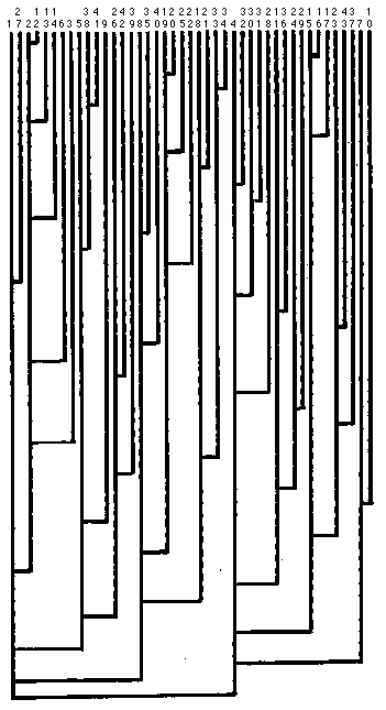

Fig.3 Dendrogram of cluster analysis

Conclusion

Using the cluster analysis, several samples that were seized from one suspect formed the same group. Further, even if the different suspects purchased from the same seller, the samples belong to the same group and the relation between the suspects and sellers becomes apparent. The cluster analysis was used to compare the similarity between samples, and with the use of a personal computer, the analysis was performed quickly and more easily.

References

1) D.G. Kleinbaum, L.L. Kupper and K.E. Muller. Applied Regression Analysis and Other Multivariate Methods, PWS-KENT Publishing Company, Boston, 1988.
2) C. Chatfied and A.J. Collins. Introduction to Multivariate Analysis. Chapman & Hall Ltd., London, 1988.
3) M. Hida, T. Mitsui and Y. Fujimura. Identification of unknown synthetic resin by means of multivariate analysis of pyrograms. Nippon Kagaku Kaishi. 6: 972-6 (1989).
4) T. Mitsui, M. Hida, and Y. Fujimura. Searching of medicines from pyrograms using personal computer. Eisei Kagaku. 36: 226-33 (1990).
5) T. Mitsui, M. Hida, and Y. Fujimura. Identification of fibers by means of multivariate analysis of pyrograms. Bunseki Kagaku. 39: 427-31 (1990).

Return