Computer Simulation of Hydrodynamic Models for Chemical/Pharmaco-Kinetics
Setsuro SUGATA and Yoshihiro ABE
 Return
1 Introduction
In chemical/pharmaco-kinetics, the variation in concentration (amount) of a drug with time is generally represented by a 2-dimensional graph (x-axis = time, and y-axis = concentration; refer to texts [1, 2]). Although this kind of graph is essential for studying kinetics, it is not sufficient for a thorough understanding. Simulations of these kinetics using the hydrodynamic models [3 - 13]make up for the insufficiency of the 2-dimensional graph. The merit of studying kinetics with hydrodynamic models has been recognized because the following are directly observable: the difference in water levels between two vessels connected by a capillary (if one edge of the capillary is free, water level from the edge) is the driving force of the hydrodynamic model, and equal water levels represents an equilibrium state. Although simulation using actual hydrodynamic models is not difficult, the preparation of the desired conditions for the vessels, capillaries and so on are rather difficult, and the simulations need rather a lot of time. In this study, six hydrodynamic models of typical linear chemical/pharmaco-kinetics (one example containing a zero-order process), accompanying a 2-dimensional graph of the time-course variations, were simulated by computer.
2 Theory
Two actual hydrodynamic models are shown in Figure 1 schematically; the six simulated models were obtained by combining the two basic models and the zero-order model. In the figure, the volume of water, VA, in a vessel corresponds to the concentration of reactant (in chemical kinetics), or the amount of drug in a compartment (in pharmacokinetics). Similarly, VB corresponds to the concentration of product (in chemical kinetics), or the amount of drug eliminated into urine and bile or dispersed into another compartment (in pharmacokinetics). In the figure, VA + VB = Vt (const.).
The flow of water in a sufficiently long capillary represents laminar flow, and is governed by Poiseuille's law [14]. According to this law, the flow rate, Q, is proportional to the water level (or difference in water levels), h, and inversely proportional to the length of the capillary, L (Figure 1). Therefore,

In this equation, a remains constant if the temperature of water and the radius of the capillary remain constant [14].
If the vessel is cylindrical (Figure 1a), h can be represented by VA as follows,

where SA is the cross-sectional area of the reactant vessel. Substituting Eq.2 into Eq.1 gives

If a/SAL remains constant during the hydrodynamic process, it can be substituted by k, where:

Equation 3 is substituted with Eq.4, and can be represented by a differential equation as follows:

Equation 5 suggests that a cylindrical vessel can be used as a hydrodynamic model of the first-order irreversible reaction [3, 4, 6, 7, 10], and k is the rate constant.
If two cylindrical vessels are connected by a capillary (Figure 1b), h can be represented as follows:

Substituting Eq.6 into Eq.1 gives

If a/SAL and a/SBL remain constant during the hydrodynamic process, these can be substituted by k1 and k2, respectively, where:

Equation 7 is substituted with Eqs.8 and 9, and can be represented by a differential equation as follows:

Equation 10 suggests that the apparatus shown in Figure 1b can be used as a hydrodynamic model of the first-order reversible reaction [6], and k1 and k2 are the rate constants of forward and reverse processes, respectively.
If the capillary in Figure 1a is very long, and is almost vertically suspended, the magnitude of Q will be kept almost constant during the hydrodynamic process. Thus, the suspended long capillary model can be a good zero-order hydrodynamic model [10]. Because of the limited presentation area, however, the suspended long capillary model is impractical for a realistic presentation in the computer simulation. Therefore, another simple model was chosen for the zero-order hydrodynamic model in the computer simulation. In the simple model [9], the water surface in Figure 1a is pushed by a sufficient excess of pressure so that the magnitude of Q can be kept constant. This can be represented by a differential equation as follows:

Equation 11 suggests that the simple model can be used as a hydrodynamic model of the zero-order irreversible reaction, and k is the rate constant.
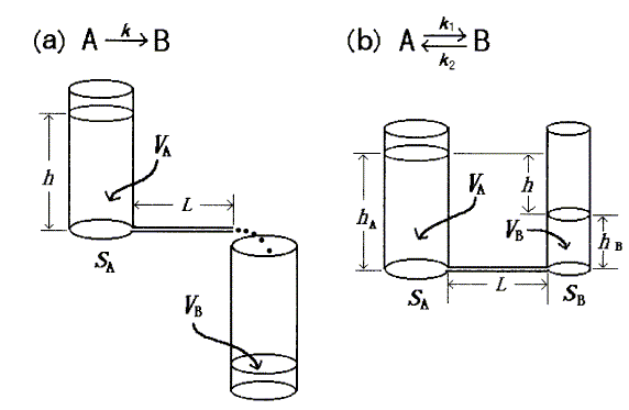
Figure 1. Schematic presentation of the two actual hydrodynamic models, which are components of the six simulated linear chemical/pharmaco-kinetic models presented here.
3 Methods
Computer simulations for the hydrodynamic models were performed using an NEC Model PC-9801/9821 personal computer with a program written in BASIC (N88BASIC(86)). The program is available on request from the committee of software distribution of The Chemical Software Society of Japan (CSSJ).
The flowchart for the simulation is shown in Figure 2. All calculations for the simulations were performed using the integral rate laws [1, 2, 16]. If necessary, the simulation can be stopped at predetermined intervals. For reference, the reaction progress is represented by an ordinary line graph. If you input new parameters of rate constants (k1, k2, k3), time duration of simulation (T2), number of calculations (NC), and capital letter "Y" at the question "add log plots (Y/N) ?", the initial parameters are replaced by the new parameters and semi-logarithmic presentation is added to the graph; if you select default values, the initial parameters are maintained. To change other parameters, it must be done in the program directly.
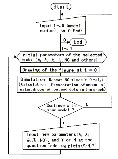
Figure 2. Flowchart for the computer simulation of hydrodynamic models for chemical/pharmaco-kinetics.
For the first-order irreversible process (Figure 1a), the variation in k value in Eq.4 is accomplished by changing the value of L; the values of S of all cylinders in a model are the same and are kept constant. For the first-order reversible process (Figure 1b), the variation in k1 value in Eq.8 is accomplished by changing the value of L (the value of SA is kept constant), and that of k2 in Eq.9 is accomplished by changing the value of SB (the value of L varies according to the value of k1). For the zero-order irreversible process , the variation in k value in Eq.11 is accomplished by changing the pressure.
In the irreversible process, a trace of the drop discharged horizontally from the head of a capillary is represented by a parabolic curve [15] (Figure 1a and 3). The magnitude of Q is represented as the horizontal range during the drop fall for a fixed vertical distance (Figure 3). On the other hand, in the reversible process, the direction and magnitude of Q are represented as the direction and length of the arrow (Figure 3). Of course, the direction and magnitude of Q change to accompany the reaction progress.
4 Results and discussion
The simulated models are (1) A ® B, (2) B ¬ A ®C, (3) A ® B ® C, (4) AÞ B ® C, (5) A Û B, and (6) C ¬ A Û B; where, Þ, ®, and Û present zero-order irreversible, first-order irreversible and first-order reversible processes, respectively. Models 1-3 are familiar in both chemical and pharmaco-kinetics [1, 2, 16]. Model 4 (one-compartment open model with zero-order absorption and first-order elimination) and model 6 (two-compartment open model with rapid intravenous injection) are characteristic for pharmacokinetics [2], and model 5 (first-order reversible reaction) is characteristic for chemical kinetics [1, 16].
Figure 3 is a simulation scene of model 6 [2]. After a drug is introduced into the plasma compartment (cylinder A) by bolus intravenous injection, it starts to disperse in the tissue compartment (cylinder B). Simultaneously, the drug is eliminated (excreted or metabolized) from the plasma compartment into urine and bile (cylinder C). At the start, both the dispersion and elimination rates are high; this is seen from the large values of h in the simulation. Therefore, rapid net loss of drug from the plasma compartment, and a rapid decline in plasma concentration, occur; this period is called the a-phase. After a certain time period, the drug will equilibrate between the two compartments (end of a-phase). This equilibrium is clear in the simulation from equal water levels; strictly speaking, complete equilibrium is observed only momentarily, then a slight deviation from equilibrium is observed continuously (left in Figure 3). Around the equilibrium, a steady-state is observed in cylinder B. Once equilibrium is reached, the rate of drug loss from the plasma compartment is reduced (start of b-phase). Drug from the tissue compartment goes back to the plasma compartment, as represented in Figure 3. The larger both k1 and k2 values in Figure 3 are, the faster equilibrium is attained (the a-phase becomes shorter), and the smaller the deviation from the equilibrium becomes. If both k1 and k2 values in Figure 3 are decupled (k3 is kept constant), the a-phase is greatly shortened; this can be regarded as a one-compartment model. In the actual hydrodynamic model, this 1:10 capillary length ratio experiment is impractical under the conditions "sufficiently long capillary"(see section 2). The longer the capillary, the slower the flow rate Q.
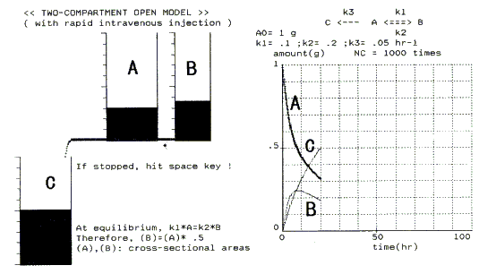
Figure 3. A scene of the computer simulation of a hydrodynamic model for chemical/pharmaco-kinetics exemplified by the two-compartment open model with rapid intravenous injection. For details, see text.
In model 5, a clear equilibrium state was observed when t = ¥. Steady-states were observed in the B cylinders of models 3 and 4 [1, 2, 16]. In each simulation, this was easily seen from equal magnitudes of Q in both in- and out-going capillaries of the B cylinder. The other two hydrodynamic models were also simulated easily and realistically.
5 Conclusion
In all computer models, the hydrodynamic models were simulated easily and realistically. The following were directly observable: ( i ) the difference in water levels (h) between two cylinders connected by a capillary (if one edge of the capillary is free, water level from the edge) is the driving force of the hydrodynamic model, and the flow rate (Q) is proportional to h; ( ii ) equal water levels represents an equilibrium state; and ( iii ) the same magnitudes of Q in both in- and out-going capillaries for one cylinder represents a steady-state. As the computer simulation can simultaneously show the ordinary graph of the variations in drug concentration versus time, it is superior to actual hydrodynamic models in studying chemical/pharmaco-kinetics.
References
[ 1] Atkins, P.W., Physical Chemistry, 5th ed., Oxford University Press, Oxford (1994), chap. 25.
[ 2] Welling, P.G., Pharmacokinetics: processes, mathematics, and applications, 2nd ed., American Chemical Society, Washington (1997), chap.13-19.
[ 3] Lemlich, R., J. Chem. Educ., 31, 431 (1954).
[ 4] Hecht, K., School Sci. Rev., 41, 439 (1960).
[ 5] Weigang, O.E.Jr., J. Chem. Educ., 39, 146 (1962).
[ 6] Lago, R.M., Wei, J. and Prater, C.D., J. Chem. Educ., 40, 395 (1963).
[ 7] Meiners, H.F.(Ed.), Physics: Demonstration Experiments, Ronald Press, New York (1970), p.1240.
[ 8] Vaidhyanathan, V.S., J.Pharm.Sci., 64, 88 (1975).
[ 9] Davenport, D.A., J. Chem. Educ., 52, 379 (1975).
[10] Asahi, Y., Yakugakusei-no-tameno-sokudoron-ensyuu (Japanese), Hirokawa Publishing Co., Tokyo (1984).
[11] Ricci, R.W. and Van Doren, J.M., J. Chem. Educ., 74, 1372 (1997).
[12] Katzung, B.G.(Ed.), Basic & Clinical Pharmacology, 7th ed., Appleton & Lange, Stamford (1998), p. 38.
[13] Sugata, S., ACH-Models Chem., 136, 349 (1999).
[14] Munson, B.R., Young, D.F. and Okiishi, T.H., Fundamentals of Fluid Mechanics, 2nd ed., Wiley, New York (1994), p.456.
[15] Tippens, P.E., Physics, 5th ed., McGraw-Hill, New York (1995), p. 119.
[16] Tebbutt, P., Basic Mathematics for Chemists, 2nd ed., Wiley, Chichester (1998), p. 174.
 Return

 Return


 Return